What are wildcard characters in Excel?

Wildcard characters in Excel are special characters that can be used to take the place of characters in a formula. They are employed in Excel formulas for incomplete matches.

Excel supports wildcard characters in formulas to return values that share the same pattern. The characters are used to look for a text string with the same known patterns — the beginning and the ending characters, and also, the number of characters presented in the cell.

Wildcard characters are useful especially when the exact cell content is not known. It’s important to note that they only work with text, not numbers.

Types of wildcard characters

 There are three wildcard characters: 

* (asterisk)

? (question mark)

~ (tilde)

Asterisk

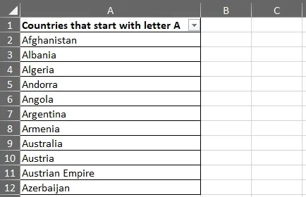
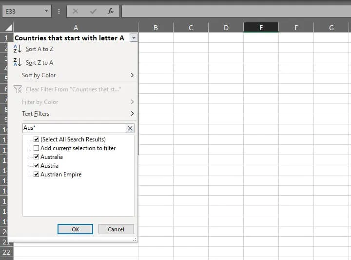
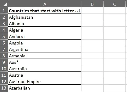
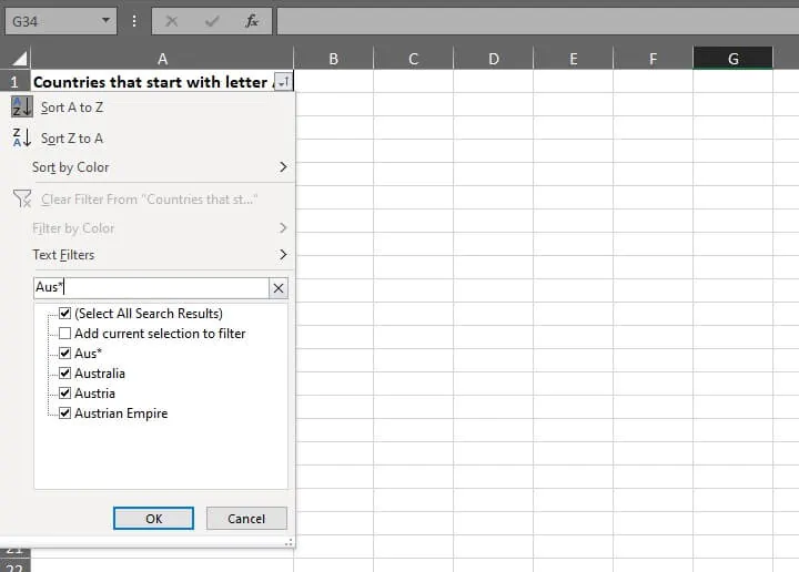
* (asterisk) represents any number of characters. For example “Aus*” returns Australia or Austria. 

Question mark

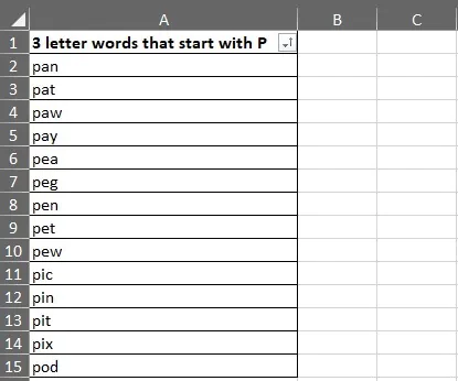
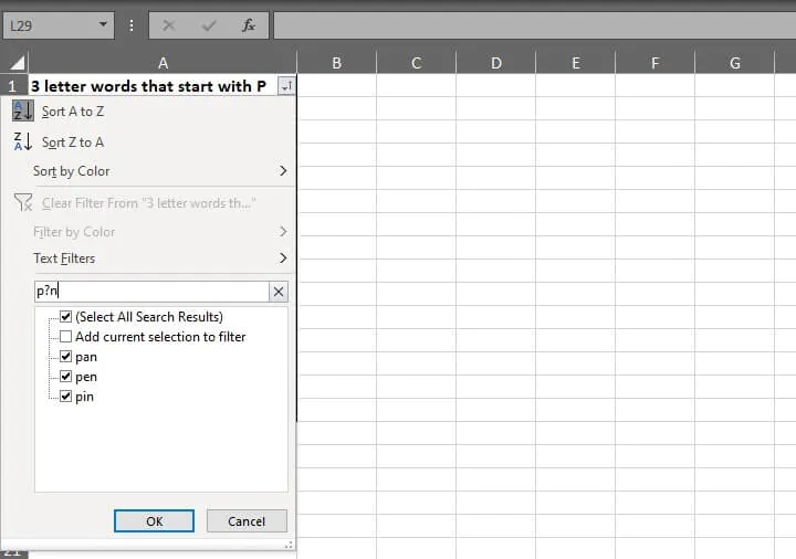
? (question mark) represents one single character. For example, “p?n” returns pan, pen or pin.

Tilde

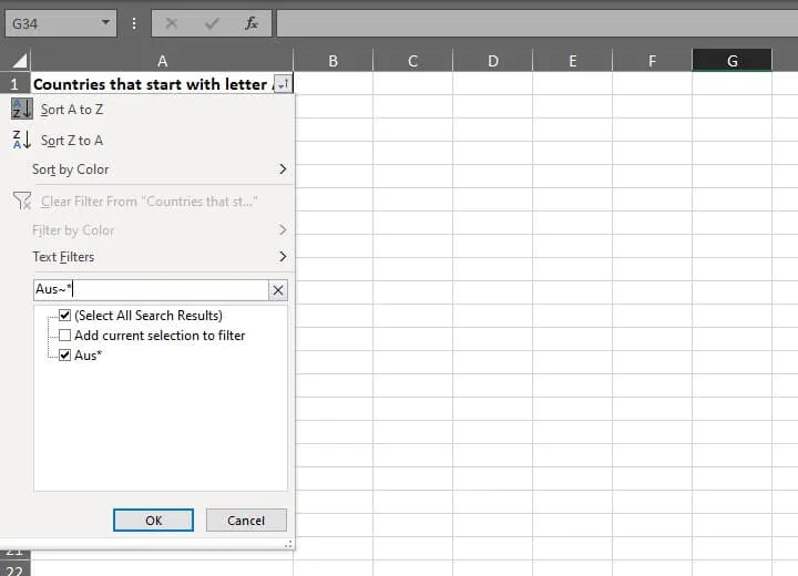
~ (tilde) is used to literally indicate the asterisk and question mark characters as they are, as * or ?, instead of a wildcard character in the formula. For example, “Aus~*” returns Aus* but not Australia or Austria like above.

How to use wildcard characters

Wildcard characters are commonly used in some basic Excel formulas, i.e., COUNTIF, COUNTIFS, VLOOKUP, FIND AND REPLACE, SEARCH, CONDITIONAL FORMATTING, etc.

Here are some examples of how it works:

1. VLOOKUP

In a normal circumstance, VLOOKUP looks up the exact value specified in a list and returns the corresponding value in a table.

Sometimes, the exact, full value in the list is not available and only the partial content is known. This is where wildcard characters come in handy.

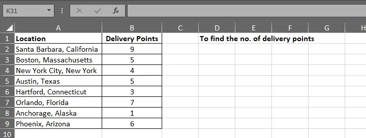
In the example below, the task is to find out the number of delivery points for Austin. But instead of Austin, the list displays Austin, Texas.  

The usual VLOOKUP formula wouldn’t work in this scenario because the lookup value – Austin, does not have the exact match.

 To find the information, enter: 

=VLOOKUP(D3&”*”;A1:B9;2;FALSE)

By inserting “*”, it tells Excel to look for any text that begins or ends with the lookup value in D3 – Austin, and it may have any number of characters after the text.

It finds an exact match, which is 5 in this case.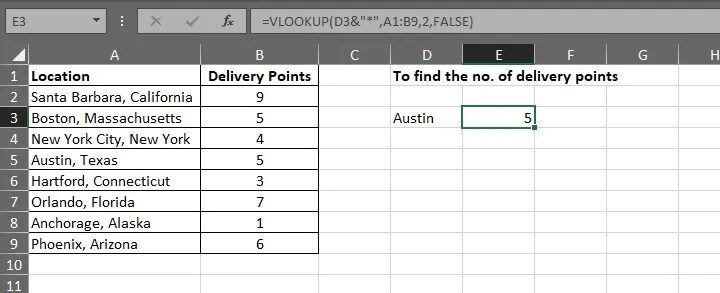 

2. FIND AND REPLACE

Using wildcard characters in Excel find and replace is useful to correct data and make the data set consistent throughout the database.

This situation is particularly common when handling data entered manually, either by staff or customers, creating extra values in the database and could make analysis difficult.

The example below shows a common picture when handling a client’s database.

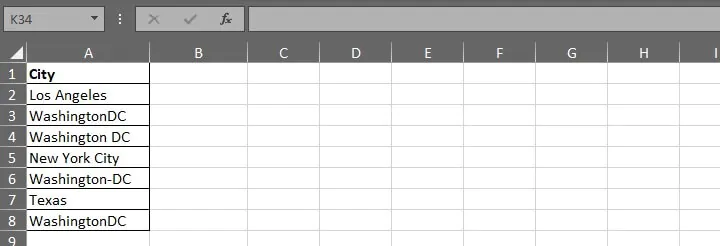The cities under Washington DC could be confusing.

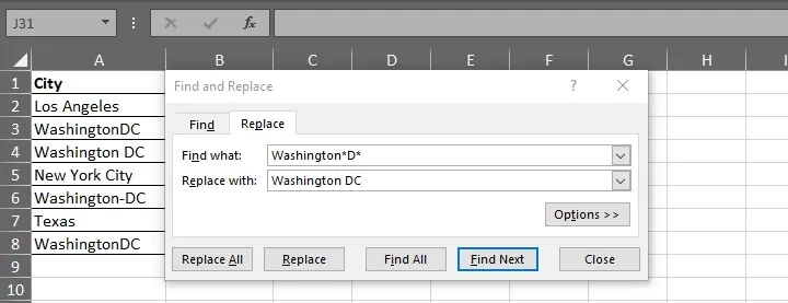
To rectify, use the simple “FIND AND REPLACE” function in Excel.

• Find Washington with a D after it and replace it as “Washington DC” 

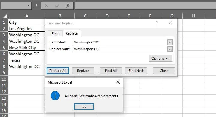
• Click “Replace All” and now all the “Washington DC” values are aligned, resulting in a clean database. 

3. COUNTIF

To include wildcard characters as part of the COUNTIF function counts the number of cells in the given range that meets the specified number of characters.

• i.e., there’s a list of country codes, and the task is to count the number of countries with three characters in their respective country code.

In this scenario, each ? refers to one character. 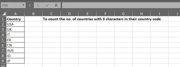Since we would like to find out the country with three characters in their country code, the formula should include three ???

To find out, enter: 

=COUNTIF(A2:A9;”???”)

The return value is 2.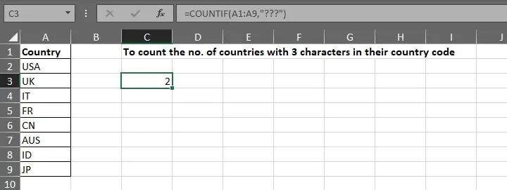 

4. CONDITIONAL FORMATTING

In addition to formulas, wildcard characters can be used to create conditional formatting as well. 

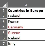
Say, the task is to highlight the countries with names that begin with the letter G. 

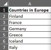
1. Go to Conditional Formatting > New Rule > Select “Use a formula to determine which cells to format.”
2. Input the formula below. 

The idea is to find countries with names that begin with the letter G. So * (asterisk) is used to request Excel to return values that begin with G and are followed by any number of characters.

3. Select the desired formatting — in this case, font in red. 

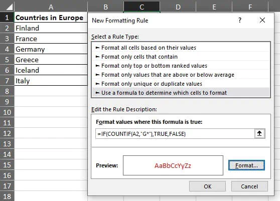
4. Click Okay, then apply the same format to the rest of the cells under Column A by using Format Painter. 

The result is below:

Excel wildcard not working? Here’s why

Mentioned previously, the use of * (asterisk) and ? (question mark) refer to different situations. However, they don’t work if the wildcard characters themselves are part of the lookup value.

• i.e., to find “Aus?”, “Aus~?” is required. 

Summary

Wildcard characters work best in situations where the given data is incomplete or partially available. They are used to take the place of characters in a formula, whether as any number of characters or a single character, expressed as * (asterisk) and ? (question mark). 

These characters are compatible with the following functions:

• AVERAGEIF, AVERAGEIFS
• COUNTIF, COUNTIFS
• SUMIF, SUMIFS
• HLOOKUP, VLOOKUP, XLOOKUP
• MATCH, XMATCH
• SEARCH

CONDITIONAL FORMATTING also supports wildcards. Wildcards help search, match, and return a partial match in situations where the lookup value is incomplete. They sometimes rectify data by synchronizing them as well.